Path Planning Project
In this project I implemented the C++ algorithms for a car to drive safely on a highway simulation with other cars driving a different speeds. My car manages to adapt to the highway traffic, change lanes when safe in order to drive faster, while keeping below the 50 MPH speed limit and within its lane.
The goals for the project are described in the Project’s Rubric:
- The code compiles correctly.
- The car is able to drive at least 4.32 miles without incident.
- The car drives according to the speed limit.
- Max Acceleration and Jerk are not exceeded.
- Car does not have collisions.
- The car stays in its lane, except for the time between changing lanes.
- The car is able to change lanes
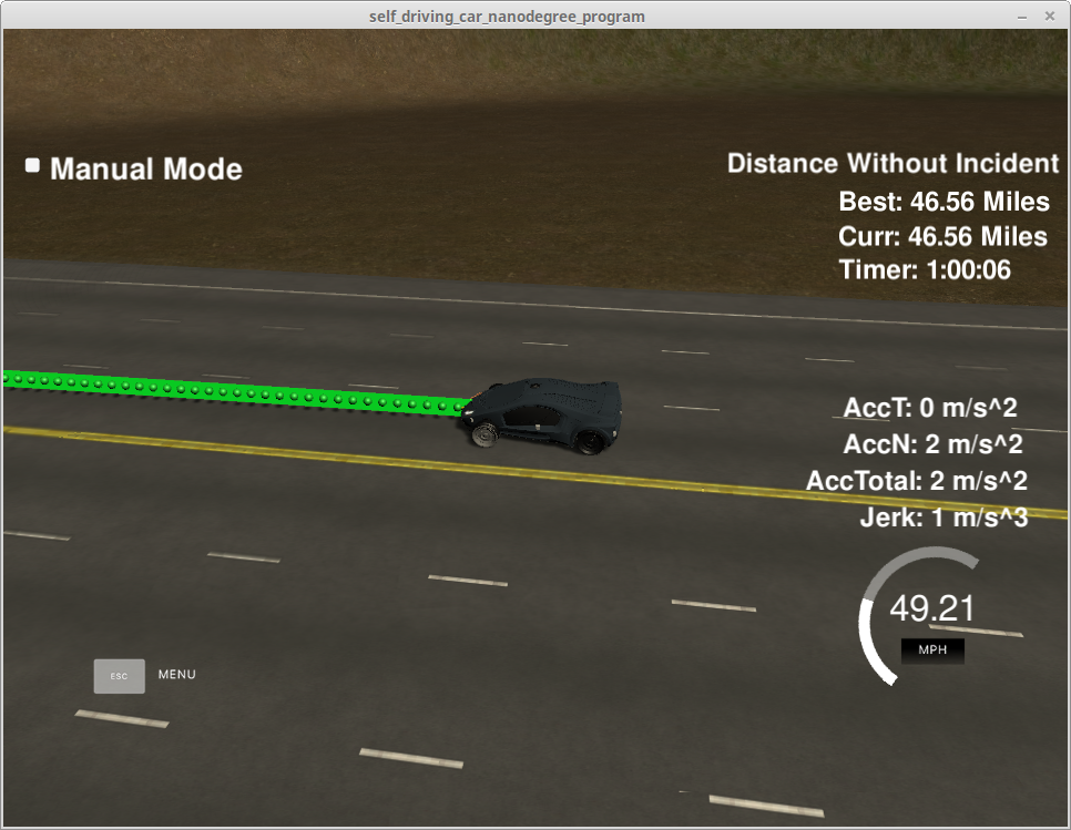
All the goals were fulfilled in the final implementation of the code, and the vehicle was able to drive for more than an hour without incidents. The code can be found on the GitHub repository
The main part of the code was implemented in main.cpp, while some functions where placed in helpers.h to improve readability and modularity to the code.
main.cpp
At the beginning of main.cpp, before its main() function, I declare a data structure to store the relevant variables to our car’s state. This will be used later in order to plan the car’s behavior using a finite state machine.
struct Car{
  int pred_lane;
  int goal_lane;
  double pred_vel;
  double goal_vel;
  string state;
};
At the beginning of the main() function the car’s state is initialized.
The architecture to communicate with the simulator is already given here. The central part of the program begins when the simulator delivers data from line 97: if (event == "telemetry") {
After this the data coming from the simulator is stored in several variables and the vectors used to deliver the next path locations to our car are declared:
vector<double> next_x_vals;
vector<double> next_y_vals;
From here begins my own implementation of the code. The structure of my code can be broken down in:
- Prediction of the future position of my car and other cars on the road
- Behavior Planning of my car using costs functions to evaluate which lane to use
- Trajectory Generation to accelerate, keep in lane speed, and change lanes, keeping low levels of jerk and acceleration
Additionally the code contains several print out statements that were used to understand and debug the behavior of the different variables as the road conditions were changing. These statements are signaled by comments and are left as additional information.
Prediction
On each cycle the code will feed a series of 50 path points to the simulator for our car to follow. Not all of this positions will be realized at the end of the cycle, and the simulator will feed back the previous path points that were left over. I want to add path points from the last of the previous path position. This is a position in the future of my car that I calculate and it is from this predicted position that I refer the rest of the operations to decide the future planning and trajectory.
On the first cycle there will be of course no path leftover and the initial position will be taken as the predicted position.
The quantities of interest are the last position on Frenet coordinates, the last and the one before last positions of the previous path in map x, y coordinates. From these last two positions I calculate the car’s angle and its velocity. Having these two points will also be necessary to generate the next trajectory using the spline curve.
pred_x = previous_path_x[path_size-1];
pred_y = previous_path_y[path_size-1];
pred_x2 = previous_path_x[path_size-2];
pred_y2 = previous_path_y[path_size-2];
pred_phi = atan2(pred_y-pred_y2,pred_x-pred_x2);
double last_dist = sqrt(pow(pred_y-pred_y2,2) + pow(pred_x-pred_x2, 2));
car.pred_vel = last_dist/0.02;
pred_s = end_path_s;
pred_d = end_path_d;
Finally I also calculate predicted car lane and a boolean flag that indicates whether the car is currently changing lanes.
car.pred_lane = pred_d / 4;
bool changing_lanes = (car.pred_lane != car.goal_lane);
The following section of the code refers to predicting the others cars positions when my car is at the predicted point. I will use this information to determine, for each lane, whether there is a car near me, either on the back or at the front, and based on this the maximal speed allowed at each lane.
First I reduce the amount of calculation by storing in the vector cars_in_lane only the cars closest than 50 meters on the front or behind. Next I loop over this vector and choose the closest one on the front or behind, and store its distance from my car and velocity in the vectors:
vector<double> front_car_dist(3, 500);
vector<double> back_car_dist(3, 500);
vector<double> front_car_vel(3, -1);
vector<double> back_car_vel(3, -1);
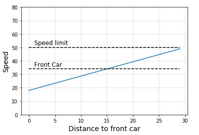
Having the distance and speed of the closest car in front of us on each lane, we can determine the maximal speed that our car will be able to drive on each lane. My first attempt was to set this velocity equal to the car in front of me, but this wasn’t realistic and dynamic enough for some cases that I encountered on the simulator. So, I finally set the speed with the following formula: when the next car is 30m in front I began to adapt my speed to it linearly so that I set its same speed when it is 15 meters in front of me. If the distance if further reduced for some reason I continue this linearity down to an even lower speed that the car in front of me has. That way I will expand the buffer back to the 15m safety distance.
This formula can be expressed as a linear function Y = X * A + B, with the indexes A and B properly chosen as shown in the code snippet below.
for(int check_lane = 0; check_lane<3; ++check_lane){
  if(front_car_dist[check_lane] < 30){
    double A = (speed_limit - front_car_vel[check_lane]) / 15;
    double B = 2*front_car_vel[check_lane] - speed_limit;
    max_speed[check_lane] = A * front_car_dist[check_lane] + B;
  }
  else{
    max_speed[check_lane] = speed_limit;
  }
}
Behavior Planning
For planning and setting behavior I use a finite state machine. This describes the three possible states the car can be in: Keep Lane (KL), Lane Change Left (LCL), and Lane Change Right (LCR). As the car finds itself in one of these states, and a certain lane, other states will be available for it to change to. As expressed by the code below, a car can always choose KL as its next state. If it is in KL, depending on the lane it’s in it can choose to transition to LCL or LCR states. If it is in LCL or LCR it can keep this state or change to KL.
vector<string> states;
states.push_back("KL");
if(car.state == "KL") {
  if (car.pred_lane != 0) { states.push_back("LCL"); }
  if (car.pred_lane != 2) { states.push_back("LCR"); }
}
else if (car.state == "LCL") { states.push_back("LCL");}
else if (car.state == "LCR") { states.push_back("LCR");}
The finite state machine could contain more states. For example Prepare Lane Change Left (PLCL) and Prepare Lane Change Right (PLCR) were used in the lesson. Also other states will be useful to describe a more complex environment than highway driving. However, these three states were already very efficient to perform a good navigation in the simulated highway.
After knowing which states are available for the next cycle, the decision which one to choose is taken using cost functions. These functions will assign a total cost to each state and the state with lower cost will be the most favorable to choose.
The cost function is placed in the file helpers.h, in the calculate_cost() function. The total cost is given by the addition of four cost components:
-
Efficiency cost: penalizes states in lanes with lower speeds, that have cars on it, even if they still don’t limit our speed, and favors changing to the middle lane if the next one is empty.
This last component contribute to avoid situations where our car is stuck in the lateral lane by a slow car and a slightly slower car in the center lane. Even when changing to the center lane will not makes our car drive faster, the presence of the other empty lane to the side reduces the cost of this option, as we can change to it and pass both cars.
double eff_cost = (speed_limit - max_speed[next_lane]) / speed_limit;
if(front_car_dist[next_lane] < 100)
  eff_cost += 0.04;
if (next_state!="KL" && next_lane==1 && max_speed[1] < (speed_limit -5)){
  if(  (next_state=="LCL" && max_speed[0] == speed_limit && back_car_dist[0] > 5)
    || (next_state=="LCR" && max_speed[2] == speed_limit && back_car_dist[2] > 5))
    eff_cost -= 0.15;
}
- Security cost: penalizes a state if other cars are too close to us either on the front or behind. In practice this cost is relevant to decide whether it is safe to change lanes.
double sec_cost = 0;
double sec_dist_front = 7.5;
double sec_dist_back = 5;
if(front_car_dist[next_lane] < sec_dist_front){
  sec_cost += (sec_dist_front - front_car_dist[next_lane]) / (sec_dist_front*2);
}
if(back_car_dist[next_lane] < sec_dist_back && next_lane != current_lane){
  sec_cost += (sec_dist_back - back_car_dist[next_lane]) / (sec_dist_back*2);
}
- Lazy cost: A small cost that discourage the car to change state with no reason. In case two states have the same cost, our car will prefer to keep its current state.
- Keep Action cost: If the car is currently in the middle of changing lanes, to abandon LCL or LCR state is penalized. This eliminates doubt in the middle of a maneuver that can be dangerous, and only trace back if there is a big enough reason, like the security cost.
The final sum of these costs to the total cost is weighted. The security cost is given a ten times bigger weight than the other cost, as it is very important not to collide with other vehicles on the road.
Back in main.cpp, once all possible states are assigned cost, the state with the minimum cost is chosen and the car’s state is changed to the state with lower cost.
double min_cost = 100.0;
string pref_state;
for(int i=0; i<states.size(); ++i){
  if(state_cost[i] < min_cost){
    min_cost = state_cost[i];
    pref_state = states[i];
  }
}
car.state = pref_state;
Trajectory Generation
Depending on the new state chosen, the trajectory will be defined by two parameters: the goal lane we want to be in, and the goal velocity, corresponding to that lane. The logic to assign those goals is contained in helpers.h, function set_goals().
Next, the current predicted velocity is adjusted for the next cycle taking into account the new goal velocity. I simply add or subtract a certain value to the velocity in order to come closer to the goal velocity. Different values are given if the velocity is close to zero, as more acceleration can be given, and if the velocity is close to the speed limit, as I want to be sure the car does not exceed this limit. The chosen values effect a proper dynamic in our car, not taking too long to start moving, and changing speed timely according to road conditions, always keeping below the speed, acceleration, and jerk limits.
Finally, the next trajectory is calculated with the help of the spline.h library. This method is recommended in the project description as an easy off the shelf solution.
A different route would have been to calculate the route using a quintic polynomial that minimizes the jerk. This implementation was discussed in the lesson, and I explored this route too. However, there were some challenges in this implementation:
- The boundary conditions, as chosen in the lesson implementation, are {si, ṡi, s̈i} and {sf, ṡf, s̈f}. sf represents the final position where the final speed of the car is reached. However, this position still depends on the time we judge correct to finish the maneuver. This additional parameter depends also on the road conditions, and adds a level of complexity to the algorithm.
- Further boundaries conditions were not treated in the lesson, like the maximal absolute values of velocity, acceleration, and jerk. Without these, the polynomial for a Jerk minimizing trajectory normally chooses trajectories with higher speed and acceleration than allowed. How to implement these boundary conditions in the matrices operations was not clear to me.
After pondering the two options, I considered the spline implementation to be the most robust and elegant. The implementation of the algorithm follows closely the one presented in the Project Q&A by Aaron Brown.
First, some anchor points are chosen to define the spline. To ensure continuity of the curve with the previous trajectory, the two last points of the previous path are taken. Additionally, we take three points down the lane separated on 30 meters steps.
X.push_back(pred_x2);
Y.push_back(pred_y2);
X.push_back(pred_x);
Y.push_back(pred_y);
for (int i = 1; i < 4; ++i){
  double next_s = pred_s + i * 30;
  double next_d = (2 + 4 * car.goal_lane);
  coord = getXY(next_s, next_d, map_waypoints_s, map_waypoints_x, map_waypoints_y);
  X.push_back(coord[0]);
  Y.push_back(coord[1]);
}
These points are here defined on the map’s X, Y coordinates. These coordinates present a problem defining the spline, in that if the curve is almost vertical (big variation on Y, and small variation on X) the Y dependence on X will be imprecise. Being the spline a curve, it can also happen that for one value of X, two values on Y belong to the spline. To minimize this problem, we change the reference of coordinates to our own car coordinates. In this frame the spline we want to calculate is almost horizontal.
X[i] = (shift_x * cos(0-pred_phi) - shift_y*sin(0-pred_phi));
Y[i] = (shift_x * sin(0-pred_phi) + shift_y*cos(0-pred_phi));
The spline is created according to the library instructions:
tk::spline s;
s.set_points(X,Y);
And in a final loop, we add the remainder points that together with the previous path will sum a new batch of 50 points to feed the simulator. These points are spaced according to the last defined velocity:
step_dist = car.pred_vel * 0.02;
We add successively this distance to each location, convert back to map coordinates, and append to the new path:
new_car_x += step_dist;
new_car_y = s(new_car_x);
double new_x = pred_x + new_car_x * cos(pred_phi) - new_car_y * sin(pred_phi);
double new_y = pred_y + new_car_x * sin(pred_phi) + new_car_y * cos(pred_phi);
next_x_vals.push_back(new_x);
next_y_vals.push_back(new_y);
Results
The simulation runs very good using this algorithm. All points in the project rubric were achieved and the simulation was able to run up to one hour straight without incidents and with an average speed of 46.5 MPH, which demonstrates that the car was able to navigate its way around the traffic and not be stuck behind a slow driving car.