LSTM implementation in pure Python
In this post I tell about how I designed a LSTM recurrent network in pure Python.
The goal of this post is not to explain the theory of recurrent networks. There are already amazing posts and resources on that topic that I could not surpass. I specially recommend:
- Andrej Karpathy’s The Unreasonable Effectiveness of Recurrent Neural Networks
- Christopher Olah’s Understanding LSTM Networks
- Stanford’s CS231n lecture
Instead in this post I want to give a more practical insight. I’m also doing the same, in two separate posts, for TensorFlow and Keras. The aim is to have the same program written in three different frameworks to highlight the similarities and differences between them. Also, it may make easier to learn one of the frameworks if you already know some of the others.
My starting point is Andrej Karpathy code min-char-rnn.py, described in his post linked above. I first modified the code to make a LSTM out of it, using what I learned auditing the CS231n lectures (also from Karpathy). So, I started from pure Python, and then moved to TensorFlow and Keras. You may, however, come here after knowing TensorFlow or Keras, or having checked the other posts.
The three frameworks have different philosophies, and I wouldn’t say one is better than the other, even for learning. The code in pure Python takes you down to the mathematical details of LSTMs, as it programs the backpropagation explicitly. Keras, on the other side, makes you focus on the big picture of what the LSTM does, and it’s great to quickly implement something that works. Going from pure Python to Keras feels almost like cheating. Suddenly everything is so easy and you can focus on what you really need to get your network working. Going from Keras to pure Python feels, I would think, enlightening. You will look under the hood and things that seemed like magic will now make sense.
LSTM in pure Python
You find this implementation in the file lstm-char.py in the GitHub repository
As in the other two implementations, the code contains only the logic fundamental to the LSTM architecture. I use the file aux_funcs.py to place functions that, being important to understand the complete flow, are not part of the LSTM itself. These include functionality for loading the data file, pre-process the data by encoding each character into one-hot vectors, generate the batches of data that we feed to the neural network on training time, and plotting the loss history along the training. These functions are (mostly) reused in the TensorFlow and Keras versions. I will not explain in detail these auxiliary functions, but the type of inputs that we give to the network and its format will be important.
Data
The full data to train on will be a simple text file. In the repository I uploaded the collection on Shakespeare works (~4 MB) and the Quijote (~1 MB) as examples.
We will feed the model with sequences of letters taken in order from this raw data. The model will make its prediction of what the next letter is going to be in each case. To train it will compare its prediction with the true targets. The data and labels we give the model have the form:

However, we don’t give the model the letters as such, because neural nets operate with numbers and one-hot encoded vectors, not characters. To do this we give each character an unique number stored in the dictionary char_to_idx[]. Each of these number is a class, and the model will try to see in which class the next character belongs. A neural network outputs the probability for this of each class, that is, a vector of a length equal to the number of classes, or characters we have. Then it will compare this probability vector with a vector representing the true class, a one-hot encoded vector (that’s its name) where the true class has probability 1, and all the rest probability 0. That’s the kind of vectors we get from the encode function.
So, when we pass a sequence of seq_length characters and encode them in vectors of lengths vocab_size we will get matrices of shape (seq_length, vocab_size). It’s very important to keep track of the dimensions of your data as it goes from input through the several layers of your network to the output, and I frequently indicate the dimensions in the code.
This will be a topic too in the other implementations. TensorFlow and Keras expect not a single input, but a batch of them. We won’t do batches here to keep it simple. In order to do the same thing in TensorFlow and Keras we will use batches of one element, and that will be one dimension more we need to keep track.
Model architecture
After having cleared what kind of inputs we pass to our model, we can look without further delay at the model itself
The four main functions making the LSTM functionality are lstm_step_forward(), lstm_forward(), lstm_step_backward(), and lstm_backward(). I programmed these functions along the lines described in the CS231n assignments. I’ll explain them below.
After these function definitions we have the main body of the program. A pseudocode description looks like:
- Load data
- Define hyperparameters
- Initialize model parameters (Wx, Wh, b, Why, by)
- While loop
	. Get next data batch
	. (Test sample with current model every N iterations)
	. Forward pass
	. Backward pass
	. Gradient update
The forward pass, backward pass, and gradient update is where the network gets trained. On the Test step we use the model to check what texts it’s able to generate as it’s trained so far. The four sections are explained below.
Forward pass
The code snippet responsible of the forward pass
    h_states, h_cache = lstm_forward(inputs, prev_h, Wx, Wh, b)
    scores = np.dot(h_states, Why.T) + by
    probabilities = np.exp(scores) / np.sum(np.exp(scores), axis=1, keepdims=True)
    cross_entropy = -np.log(probs[range(seq_length), np.argmax(targets, axis=1)])
    loss = np.sum(correct_logprobs) / seq_length
That can be represented in the following diagram:

We apply two network operations: the LSTM forward pass and the dense transformation from the hidden states to our final scores.
The lstm_forward() function will call lstm_step_forward() for each character in the input sequentially. The outputs of lstm_step_forward() are the hidden and cell states that the LSTM keeps to take into account all the previous inputs in the sequence. The hidden states, despite their name, are the external variable that get passed to the dense layer to figure out the next character from them. The cell states are internal to the LSTM and give it the ability to keep or forget past information, avoiding the exploding or diminishing gradients problem present on simple RNNs.
We set the initial hidden state to zeros before the main loop. The initial cell state is set to zeros on each call of lstm_forward(), at the beginning of each sequence.
The interesting mathematics are contained in lstm_step_forward(). This is simply an expression in Python of what you can read in Christopher Olah’s Understanding LSTM Networks.
    _, H = prev_h.shape
    a = prev_h.dot(Wh) + x.dot(Wx) + b      # (1, 4*hidden_dim)
    i = sigmoid(a[:, 0:H])
    f = sigmoid(a[:, H:2*H])
    o = sigmoid(a[:, 2*H:3*H])
    g = np.tanh(a[:, 3*H:4*H])              # (1, hidden_dim)
    next_c = f * prev_c + i * g             # (1, hidden_dim)
    next_h = o * (np.tanh(next_c))          # (1, hidden_dim)
    cache = x, prev_h, prev_c, Wx, Wh, b, a, i, f, o, g, next_c
    return next_h, next_c, cache
Inside we begin with something similar to a dense layer connection, but with two inputs and two matrices, the previous hidden state with matrix Wh, and our current character input x with Wx. And of course adding up a bias b. We obtain a vector four times the length of the hidden dimension that we divide into the four gates i, f, o, g. Finally we apply the LSTM equations to obtain the next hidden state and the next cell state.
Don’t worry now with all those variables we pass in the cache. They will be used in the backward pass.
The output of lstm_forward() is a sequence of hidden states. In the dense layer, each of these hidden states are transformed to a vector of scores of the same length as the input dimension, that is, one score for each possible output character.
scores = np.dot(h_states, Why.T) + by
As these scores are not in the best format for the next steps, we normalize them with the softmax function, giving us the probability of each possible character.
probabilities = np.exp(scores) / np.sum(np.exp(scores), axis=1, keepdims=True)
Finally, the cross-entropy values are the probability of the right character. For our sequence above (“First Citizen”), maybe the network gave the maximal probability to the character “p”, but we take the smaller probability given to the correct option “i”. The smaller the probability given to “i” the more wrong the network was. And the smaller the probability was, the bigger the -log operation will be.
cross_entropy = -np.log(probs[range(seq_length), np.argmax(targets, axis=1)])
The total sum of these cross-entropy values give the total loss.
loss = np.sum(correct_logprobs) / seq_length
So to minimize the loss, the probabilities given to the correct characters by the network should be bigger. We’ll do that in the next steps.
Backward pass
The code snippet for the backward pass is:
    dscores = probs
    dscores[range(seq_length), np.argmax(targets, axis=1)] -= 1
    dWhy = dscores.T.dot(h_states)
    dby = np.sum(dscores, axis=0)
    dh_states = dscores.dot(Why)
    dx, dh_0, dWx, dWh, db = lstm_backward(dh_states, h_cache)
The backward pass consists in applying the backpropagation method to obtain the gradients of our model parameters. We will use these gradients in the next step to minimize the loss and improve those model parameters.

Basically we want first to know how should I change the scores in order to reduce my loss. The rate of change of the loss with regards to the change of the scores is given by derivative dscores. To understand the formula of dscores above, please see this notes
But still, we cannot just change the scores. We can just change our weights Why, by, Wx, … So, we backpropagate the scores derivative through each operation we did on the forward pass until we get the derivatives of our weights. First we backpropagate through the dense layer, which gives us the derivatives of our weights Why and by, as well as the derivative of the hidden states dh_states. The equations are a simple example of backpropagation (again, more info on CS231n), and they correspond to this backpropagation diagram:

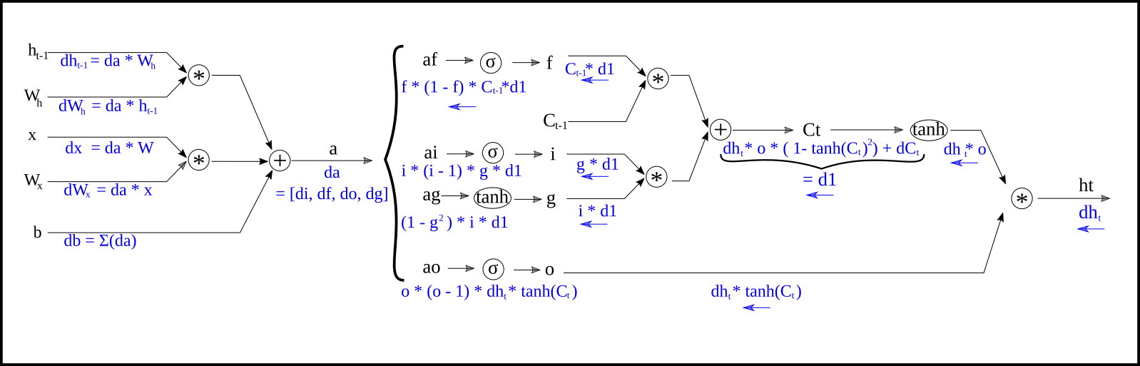
Now, the same happens with dh_state; we cannot directly change it and must backpropagate to get the gradients of our weights Wh, Wx, and b. These operations are contained in lstm_step_backward(), and this time is somewhat more complex. The code is not by itself self explanatory, I think. So, probably the backpropagation diagram will be more illustrative:
Gradient update
After we have all the derivatives we can do the gradient update. Here I apply a simple gradient descent and I subtract to each parameter its derivative multiplied by a small constant, the learning rate.
    for param, dparam in zip([Wx, Wh, Why, b, by], [dWx, dWh, dWhy, db, dby]):
        param -= learning_rate * dparam
We could have applied other rules to the gradient descent that usually work better. The different ways to apply gradient descent are called optimizers. But for educational purposes gradient descent is simple and works good enough here. We repeat this small gradient descent step over and over, updating our model parameters on each loop, until by minimizing our loss we get better and better results. The full process until here can be represented as:

Test
Of course we want to test our network and see what type of texts can it deliver. This is going to be easy. We just run the forward pass, with a random input. When we got the probabilities for the next characters, instead of comparing with any target, we’ll just pick a choice based on the probabilities. Then, if we want to sample a full text, we give this output as input for the next loop, and sample as many characters as we like.

This logic is contained in the sample() function:
def sample(x, h, txt_length):
    txt = ""
    c = np.zeros_like(h)
    for i in range(txt_length):
        h, c, _ = lstm_step_forward(x, h, c, Wx, Wh, b)
        scores = np.dot(h, Why.T) + by
        prob = np.exp(scores) / np.sum(np.exp(scores))
        pred = np.random.choice(range(input_dim), p=prob[0])
        x = aux.encode([pred], vocab_size)
        next_character = idx_to_char[pred]
        txt += next_character
    return txt
Here we basically do “manually” the process that lstm_forward() does. We call repeatedly lstm_step_forward() and keep the output prediction, hidden and cell states, to pass it on the next loop iteration. For the prediction we use the numpy function random.choice() that chooses elements in an array based on assigned probabilities. If we just choose the maximal probability the texts turn out with less variability and less interesting.
With this you will have fun watching your network improves as it learns to generate text in the same style as the input, character by character.
Summary
As you have seen, programming a LSTM in pure Python from scratch is quite an effort, and it only makes sense, in my opinion, if you want to learn all the details and mathematics of what the network really does. But that can be a very useful thing, as this post explains. I also think that TensorFlow and Keras may be more difficult to debug if you don’t know what is going on inside their functions. You can use them without knowing what gradient descent or backpropagation is, and that is great for many purposes. But it is kind like using some magic tools, and if you find some issue where the magic stops working you don’t know very well what else to try.
So, the effort of the code above may be of not much practical use, but it can pay off down the road.