Behavioral Cloning
The goal of this project is to let a neural net learn to drive by watching yourself drive in a simulator. This way the net will clone your behavior and take the same turns in the same situations as you did.
Actually, to achieve this we use a linear regression model. That differs from the classifier models frequently used in neural nets for visual recognition. Here, while we have an image as input, our output will be a continuous value for the angle we want our car to turn. We train this net to output an angle as close as the value the applied as possible on each situation.
The model was written using Keras, and the code can be found on the GitHub repository
Model Architecture and Training Strategy
1. Model architecture
I start with the model suggested in the lesson, based on the actual model used by Nvidia to train a real car to drive autonomously. I also introduced a Dropout layer to reduce the overfitting I was observing at training time.
My final model consists of a normalization and cropping layers (preprocessing), five convolutional layers, and three fully connected layers with a dropout layer after the first f.c. layer. The output of the network has dimension one, a number, which represents the driving angle the net would apply on the analyzed image. The training process will compare this value with the real angle I applied when collecting the training data.
This is a regression problem instead of a classification problem. This means that we want our value of interest (the angle), which has some error, to “regress” to the correct value, instead of being classified (as right or wrong, for example).
2. Overfitting
Overfitting occurs when the model learns to predict exactly the training data we are feeding it. This produces a model that cannot generalize well to unseen data. The overfitting can be measured comparing the accuracy on training and validation data. If the accuracy grows close to 100% on training data, but lags behind on validation data, we are experiencing overfitting.
In this case, as a regression network, we compare the loss between training and validation samples.
The most common methods to reduce overfitting are:
- Increase variability on training data, by either collecting more data cases or by artificial data augmentation
- Dropout or regularization layers. I obtained good results with one dropout layer.
- Early stopping, as the more the net trains the more it adapts to the training data at hand, leading to overfitting. Two or three epochs training seem to be a good training amount for my model.
3. Model parameter tuning
The model used an adam optimizer.
An inspection of different values of the learning rate was made, with the results plotted in the section below.
4. Appropriate training data
Correct training data aquisition was very critical (and challenging) for this project. The model is designed to just clone the behavior seen on training data. Thus, the car will only drive as good as I was able to drove.
Learning to control the car with the mouse was very important. The way the keyboard controls work, it is necessary to press and release the key to correctly modulate the driving and not steadily increase the angle out of range. This lead to a combination, within a curve, of big and zero angles, which are per se incorrent values for that frame of the road. Mouse control meanwhile, allows a steady application of the correct angle at all times (if your personal abilitiy allows)
For details about how I created the training data, see the next section.
Model Architecture and Training Strategy
1. Solution Design Approach
I chose the proposed model architecture used at Nvidia as a starting point. This arquitecture seems well fitting for this task as it relies heavily on convolutional layers, which is an advantage for models working with images. The convolutions keep the geometrical 2D characteristics of the image, that in a fully connected layer will be broken as the image gets flattened into a vector. Subsequent convolutional layers extract abstractions that represent elements on the image on a higher level.
To train the model, the data was divided into training and validation sets. The value of the validation loss tell us the efficacy of the training and possible under- or overfitting effects. Tactics to choose the learning rate and reduced overfitting are detailed in section 3 below.
2. Final Model Architecture
The final model architecture (model.py lines 18-24) consisted of a convolution neural network with the following layers and layer sizes:
| Layer | Description |
|---|---|
| Input | 320x160x3 RGB image |
| Cropping | 320x60x3 RGB image |
| Convolution 5x5 | 24 filters, 2x2 stride, relu activation |
| Convolution 5x5 | 36 filters, 2x2 stride, relu activation |
| Convolution 5x5 | 48 filters, 2x2 stride, relu activation |
| Convolution 3x3 | 64 filters, 1x1 stride, relu activation |
| Convolution 3x3 | 64 filters, 1x1 stride, relu activation |
| Flatten | |
| Fully connected | output dimension: 100 |
| Fully connected | output dimension: 50 |
| Dropout | keep_prob: 0.5 |
| Fully connected | output dimension: 1 |
3. Creation of the Training Set & Training Process
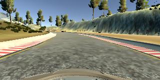
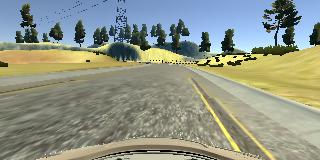
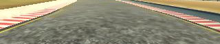
A first correct lap driving as close to the center of the road as possible is, of course, the beginning point to teach the model the correct angles to apply. Two laps were so taken, on clockwise and other counter-clockwise. Here is an example image of center lane driving:
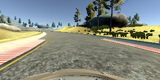
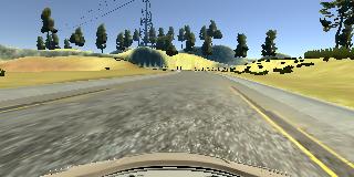
But only with this data the model will not know what to do when it begins to steer a little off the road. This can be corrected with additional laps (or part of the laps, specially at the curves) where the driving is made close to the left and right edges of the road. Examples of driving on left and right side of the road are shown below:
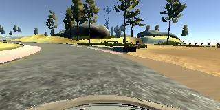
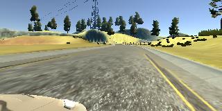
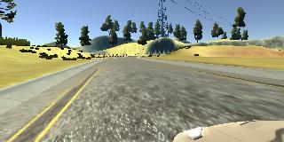
Still it could be seen that the model may drive off the road, specially at some “dangerous” parts, where the sides of the road are different as the usual (lake or dirt). To correct it more training data was acquired at these positions. This time recovery manouvers were recorded, starting almost off the road and applying the high angles needed to return to the center. A typical sequence is shown below:
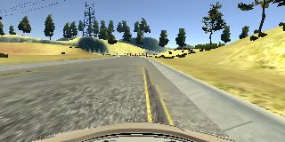
Then I repeated this process on track two in order to get more data points.
To increase data and reduce overfitting, a process of data augmentation was done by flipping the images, as follows:
The input data so acquired was feed to the model using a Python generator function and the Keras function fit_generator(), as the amount of data was big enough to make the system run out of memory. The generator includes shuffling of the data, and two generators objects, for training and validation, were defined.
The first Keras layer defined in our model, as described in last section, is a Lambda layer to preprocess the images by cropping to focus on the area of interest to our net (the road)
To train the model, the data was divided into training and validation sets. The value of the validation loss tell us the efficacy of the training and possible under- or overfitting effects.
The first parameter to be adjusted is the learning rate. Different learning rates (1e-2, 1e-3, 1e-4) showed these results:
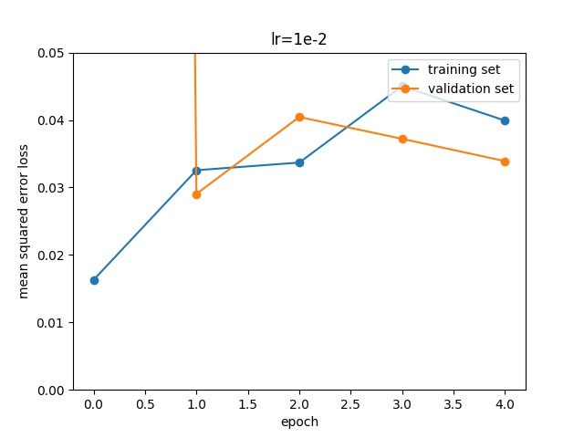
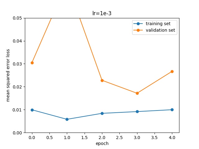
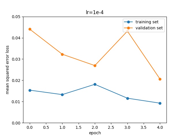
I set for a learning rate of 1e-3, that shows the best result on the training set.
However, overfitting lead to high values on the validation set. The gap between the training and validation loss could be reduced introducing a Dropout layer:
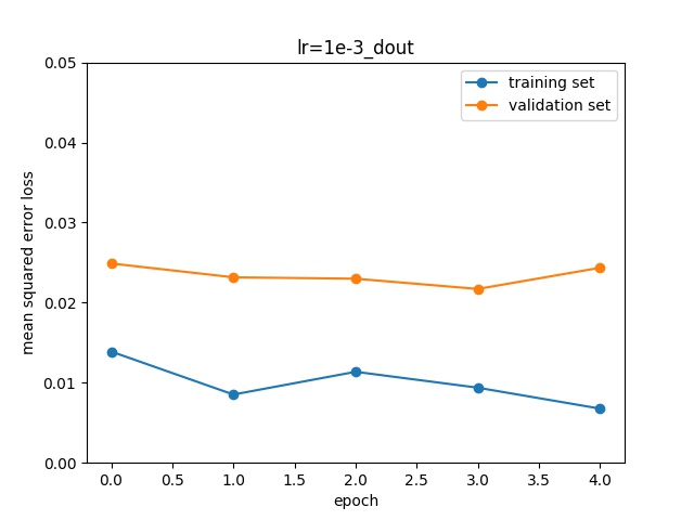
Also, more data collection, and data augmentation, as discussed above, were used to reduce overfitting. The excessive training also push the network to overfit, as seen in the plots. I choose then to limit the training to three epochs.
Simulation
Finally, a successful simulation was run and captured: